- Part 1: AI Vision Systems – The Technology Behind the Game
- Part 2: Training the AI
- Part 3: AI Vision Systems – Real-World Industrial Applications
As AI becomes increasingly embedded in every aspect of our lives, its potential to transform industrial environments cannot be overstated. In addition to cutting costs and enhancing productivity, AI vision systems play a crucial role in improving safety, for instance, only allowing access to employees wearing the correct Personal Protective Equipment.
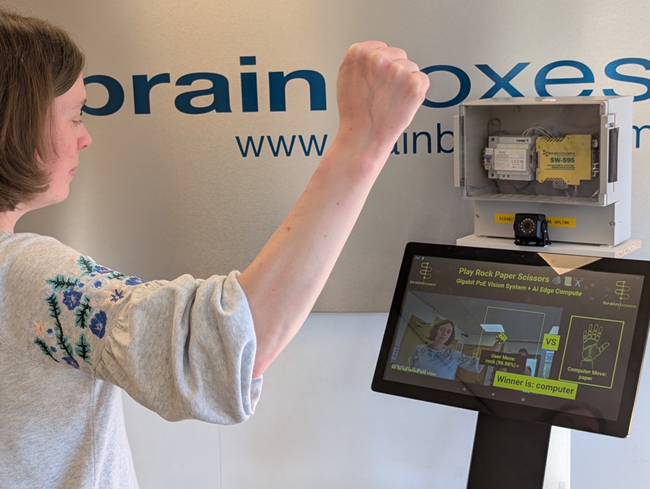
To showcase the possibilities of AI vision systems, Brainboxes developed an interactive demonstration where AI challenges humans to a game of rock-paper-scissors. This article explains the key technologies used in the system, the challenges and opportunities of using real-time AI vision systems in Industrial environments, and the importance of well-designed training protocols, inference pipelines, and edge processing.
Part 1: AI Vision Systems – The Technology Behind the Game
Whilst the game showcases the latest AI technology, demonstrating how it transforms AI vision systems, enabling them to learn from data, adapt to new conditions, and take on increasingly complex manufacturing tasks, to attract maximum attention at busy trade exhibitions, it was important to also make it interactive and fun.
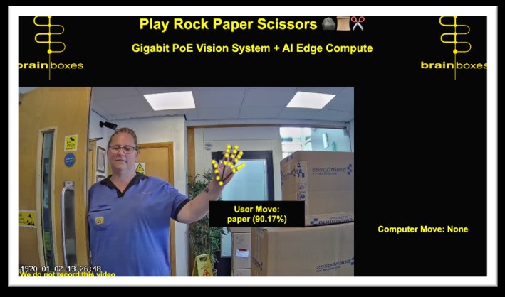
At the web-based game’s core is an AI vision system. An in-game IP camera captures the player’s hand gesture and a powerful edge-computing device, the Brainboxes BB-400, processes the information in real-time. The AI instantly recognises the player’s “move” as either rock, paper or scissors, and the computer responds with its own, determining a winner. Depending on the version of the game played, a robot arm may physically perform the computer’s move.

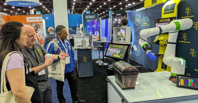
Brainboxes Rock Paper Scissors Demo Interfacing with Fanuc Robot at North American Exhibition
Key Tools: Hardware
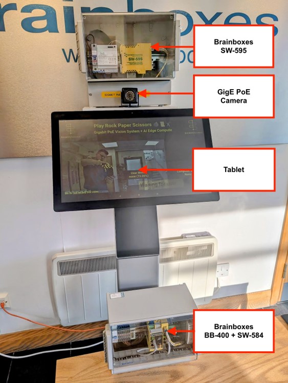
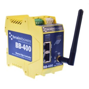
- Brainboxes BB-400: Edge processing device, based on Raspberry Pi Compute Module, with additional industrial interfaces and protection, ideal for industrial environments.
- Brainboxes SW-595: PoE Ethernet Switch, has 4 Gigabit Power Over Ethernet ports and SFP (fibre) uplink port, industrial temperature rating and dual redundant power.
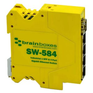
- Brainboxes SW-584: Gigabit switch + SFP, designed for reliability in industrial environments
- IP camera GigE PoE (with RTSP support): available off-the-shelf through standard distribution channels using the search term: “Mini POE IP Camera”.
- Tablet with web browser: Android or iOS-based device. Touchscreen tablet pictured is also powered by the Brainboxes SW-595 PoE switch.
- Power supplies, enclosures, DIN rail mount and cabling, additional kit required based on the system’s intended environment.
Key Tools: Open-Source Software
-
- Python: popular programming language used extensively in AI. Ties everything together and controls the game logic.
- Flask: Python webserver presents the game over the network.
- TensorFlow: Artificial Intelligence (AI) inference and training tool, originally developed by Google. This framework has been proven and matured over many years.
- LiteRT: (formerly TensorFlow Lite) generates lightweight AI models suitable to be ran on edge devices. Allows almost the same level of accuracy, but with lower memory footprint and inference time as a full AI model.
- OpenCV: Computer vision and image manipulation library original developed by Intel, used within Python. The standard way to interface with camera systems, and provide simple and efficient mechanisms for image manipulation.
- FFmpeg: Audio Video Library for streaming, encoding and decoding video. Chosen as it has many options and can also target BB-400 video hardware acceleration.
- RTSP to WebRTC: project to convert RTSP to WebRTC. Easy to use, low memory footprint and fast.
- Brainboxes has published the code to github under an MIT license get it here:

Network Topology

Note: Whilst separating the BB-400 from the tablet and camera over a fibre link is not necessary, it demonstrates that in a real-world application of the AI vision system, the edge device can be located kilometres apart with only a negligible increase in latency. This is vital to industrial environments where availability and proximity of power sources needs to be considered.
Where not required, the SW-584 and the fibre link can simply be removed, connecting the SW-595 port into the BB-400 LAN port.
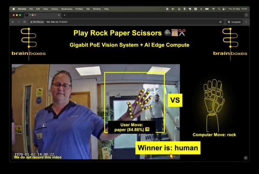
Sample demo game screen
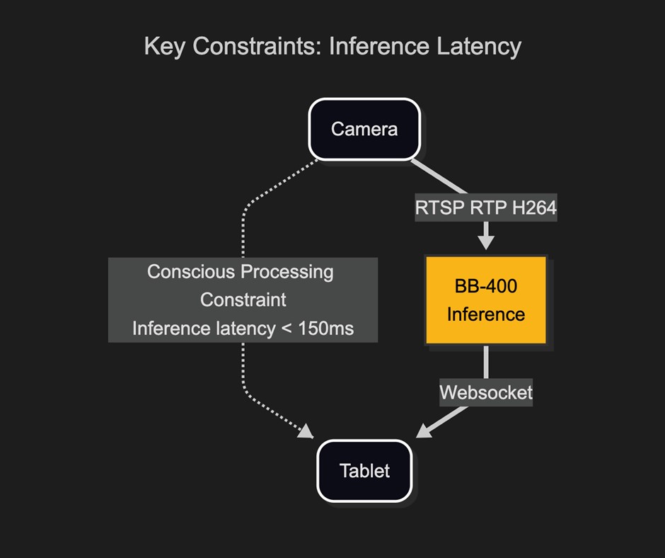
For the game to feel real, the AI vision system has to be fast. Based on human’s typical process and response times, to maintain a natural experience, the AI should present a decision within 150 milliseconds and update the video on-screen in under 70 milliseconds.
This makes it vital to minimise camera stream latency, use compact AI models for faster inference, and select efficient communication protocols.
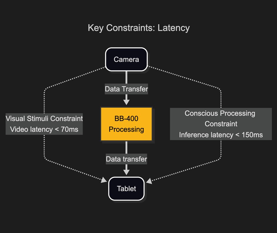
Latency is the key constraint in any real-time system
Optimising Communication: Protocols for Speed and Reliability in AI Vision Systems
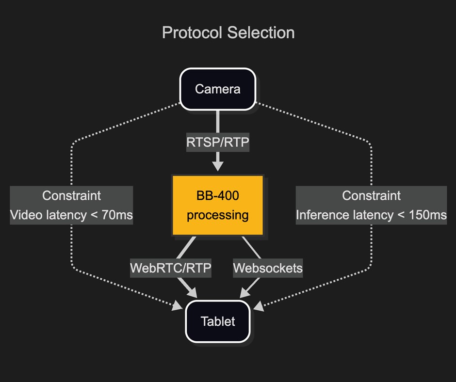
Protocol selection is key for speed and reliability
To get data from the camera to the BB-400, RTSP (Real-Time Streaming Protocol) is used. This industry standard high-level camera protocol is often used as a wrapper around RTP (Real-Time Protocol) which encapsulates the video feed.
However, the camera’s native RTSP video feed is not compatible with modern web-browsers. Several tests were made of different approaches, ultimately proxying the RTSP camera feed through the BB-400 and using the excellent Open-Source project “RTSP to WebRTC” was found to be the solution capable of high-definition resolution at sub 100 milliseconds latency.
For communicating AI prediction and game data from the BB-400 to the web-browser, WebSockets was the obvious choice. WebSockets allows for a persistent bi-directional TCP connection between the client web-browser and the Flask Webserver. As the connection is persistent, it is much lower latency than other choices within a web-browser, as TCP handshaking is only done once.
Part 2: Training the AI
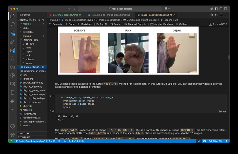
Jupyter Notebook running in VS Code to train the demo game
The first and most important step in training an AI model is to have a large, varied, correctly labelled training dataset. No amount of machine learning can correct for bad data.
Sample demo game training input
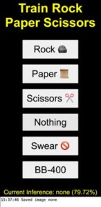
Sample demo game training screen
To achieve this, the game has a built-in data collection mode. While the game is running, a separate web-page can be opened on another device, and an admin can correctly record what gesture is being performed. The image of the gesture is then saved into the training set.
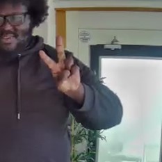
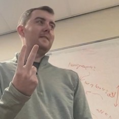
Varying the scene with differences in environmental conditions such as lighting, background and camera angles, as well as ensuring the training data includes a wide variety of player ethnicities, genders, etc., is crucial.
A good example of what to watch out for is the cultural bias we encountered when taking the demo to a North American exhibition for the first time.
Initially, the demo game AI was trained to recognise the common US variation of the ‘scissors’ gesture, with the back of the hand shown to the camera, as swearing, resulting in an error message shown to the player.
This highlights the importance of gathering diverse training data to create truly intelligent systems.
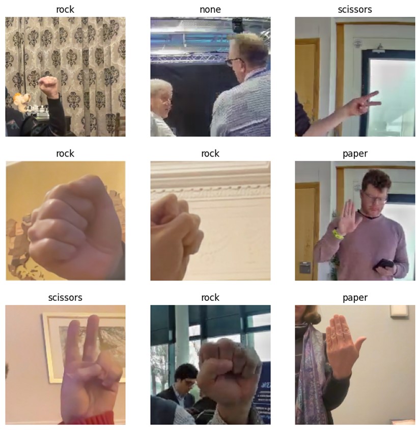
The final training data set comprised almost 2000 images across 6 categories
Setting Up the Development Environment
The demo was developed within VS Code a free Integrated Development Environment (IDE) made by Microsoft. Download here.
Note: Other IDEs are available, but untested.
As the project is Python 3 based and packages are managed by PIP, it’s crucial to ensure that the versions of different libraries are compatible with each other, the development platform, and the BB-400. To this end provided in the sample code is a requirements.txt file which should be ran with PIP, and ideally within a Python virtual environment to allow conflicting versions of packages to co-exist on your system without interfering with each other.
The project was built with Python version 3.11.9. Ensure this is installed first here.
- In Windows PowerShell:
python -m venv myenv
myenv\Scripts\Activate.ps1
pip install -r requirements.txt- In Mac/Linux terminal:
python -m venv myenv
source myenv/bin/activate
pip install -r requirements.txt- To setup Jupyter Notebooks with VS Code see here.
Now the Jupyter Notebooks within the project can be run: ensure you select the Python 3.11.9 kernel as the default.
Building an AI Model
All the information provided below can be reviewed within the source code.
In the training folder, there are 2 Python Jupyter Notebooks: both based on tutorials in the TensorFlow training documentation:
`image-classification.ipynb` which can be found here
and
`retraining-an-image-classifier.ipynb` which can be found here.
Model Selection: Sequential Model
Initially a new model (a Keras sequential model) was created and trained with the training data. The TensorFlow website has some excellent Jupyter Notebook based tutorials which can easily be run and adapted.
- Starting with a new sequential model the validation accuracy achieved was 59%.
Parameter Tuning: Image Augmentation
Image augmentation is taking an existing image and modifying it in a way that preserves the original intent, but makes the image look different. The idea is that it exposes the AI model to a more varied dataset. This may be through rotation, zoom, contrast, brightness, and flipping. Through experimentation, it was found that while augmentation was beneficial, minimal modification will achieve the maximum benefit.
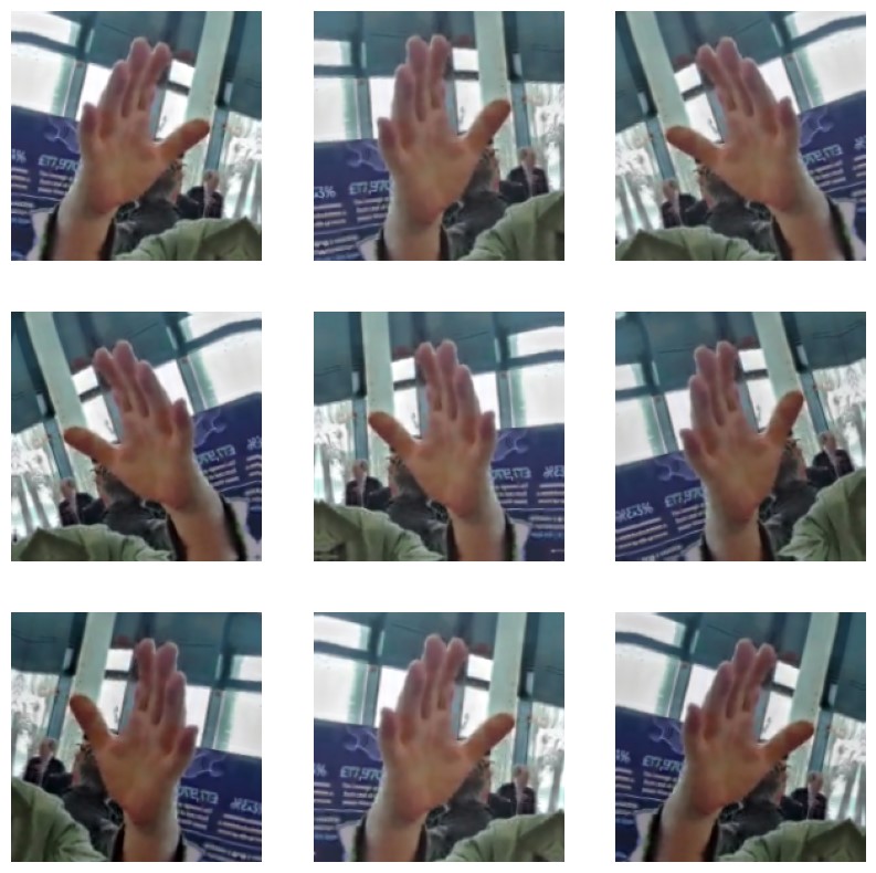
Augmented image of ‘paper’ gesture
- A new sequential model with data augmentation achieved 65% validation accuracy.
Model Selection: Transfer learning with fine tuning
Switching from a new model to a pre-trained model is where the validation accuracy really made improvements. There are many pre-trained models available online, e.g., Hugging Face 🤗, Kaggle, with each model trained against different datasets to target different aims. Within these online models there is a huge subset pre-trained for image classification, some trained with millions of labelled images across 1,000s of categories.
The idea of using a pre-trained model is not new. A pre-trained model has generalised its understanding of images, over the millions of training cycles it has undergone. As a result of the training, for example, some layers of the pre-trained model may specialise in detecting lines and curves. Subsequent layers may put these together to understand shapes like circles. Even later layers then group together different types of common objects, like wheels.
Given that the pre-trained model has a generalised understanding of imagery, applying it to our image classification needs should enable it to generalise better when recognising new Rock-Paper-Scissors gestures in the real world.
The first pre-trained model selected was EfficientNetV2.
- Applying transfer learning using the same training data as before generated a Rock-Paper-Scissors classifier with 85% validation accuracy, albeit with a model size of 23MB.
An alternative transfer learning approach was then applied to the pre-trained model, only updating a limited number of parameters by small increments, in a process known as Parameter-Efficient Fine-Tuning. This prevents the model from being distorted by the new image dataset.
- This type of fine-tuning immediately yielded an improvement to 91% validation accuracy.
Finally, MobileNetV2 (originating from as far back as 2018 – an age in AI development) was used.
- With a very small model size of 1.6MB, fine tuning achieved an acceptable validation accuracy of above 95%.
Optimisation: TFLite Quantisation
Starting with the 1.6MB model, TensorFlow Lite’s recommended optimisations were applied, additionally specifying 8-bit integer operations (which work well on the target hardware).
- This yielded a model with the high validation accuracy above 95%, and a size of just 650KB.
converter.optimizations = [tf.lite.Optimize.DEFAULT]
converter.representative_dataset = representative_dataset
converter.target_spec.supported_ops = [
   tf.lite.OpsSet.TFLITE_BUILTINS_INT8 # Target INT8 ops
]
Building the Model: Conclusion
Following a clear path and using high quality data to achieve high validation accuracy, followed by optimisation, led to an AI model which was just 650KB. It could perform inference on the BB-400 edge device in less than 45 milliseconds and had a validation accuracy of greater than 95%.
| Model | Finetune | Optimise | Validation accuracy | Size |
| Keras Sequential | 0 | 0 | 59% | 15.9MB |
| Keras Sequential | 0 | 0 | 65% | 15.9MB |
| EfficientNetV2 | 0 | 0 | 85% | 23MB |
| EfficientNetV2 | 1 | 0 | 91% | 23MB |
| MobileNetV2 | 1 | 0 | 95% | 1.6MB |
| MobileNetV2 | 1 | 1 | 95% | 650KB |
Inference Pipeline
Inference latency is key for the AI vision system demo game to feel responsive
After building the training dataset and verifying the accuracy of the trained model, the model needed to be refined to improve the latency and memory footprint. Running model inference on state-of-the-art high-speed hardware can be very different to running on a resource and power constrained edge device. The Brainboxes BB-400 hardware features the Broadcom BCM2837B0 SoC, which has quad-core 64-bit ARM Cortex-A53 clocked at 1.4 GHz and 1 GB LPDDR2 memory. While powerful for an edge device, the BB-400 must run inference, video processing, and the Rock-Paper-Scissors game webserver concurrently. While optimising inference for speed, it also had to be optimised for low CPU and memory usage.
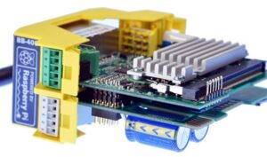
Brainboxes BB-400 Edge device runs inference and the web-based game
Before running AI inference, the incoming camera feed needed to be decoded to a frame, the region of interest extracted and then that image pre-processed to a form which suits the AI model.
Therefore, we will deal with latency for inference in 2 parts, pre-processing latency and inference latency.
Image Pre-Processing Latency
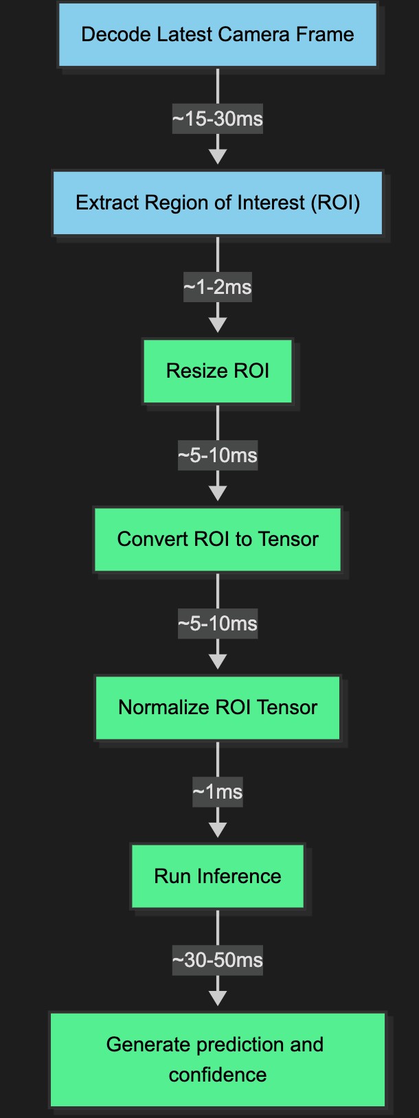
Image processing and inference pipeline
When the H264 encoded RTP video stream arrives from the camera to the BB-400, it must be processed into the correct format and data structure required by the AI inference model. This process broadly speaking contains 5 steps, in the software codebase the pre-processing is dealt with by 3 libraries:
- FFmpeg: for video stream decoding to a frame of image data
- OpenCV: for extracting the region of interest from a frame
- TensorFlow: for converting the region of interest into a data format suitable for inference.
Several optimisations were tested to achieve the lowest latency:
- OpenCV was configured to pass the hardware video decoding option on to FFmpeg.
# enable hardware decoding on BB-400
os.environ["OPENCV_FFMPEG_CAPTURE_OPTIONS"] = "video_codec;h264_v4l2m2m"- The resize algorithm used on the Region of Interest was set to nearest neighbour, which requires the least processing time to complete a resize vs other methods.
img_tensor = tf.image.resize(
   img_tensor,
   [IMG_SIZE, IMG_SIZE],
   method=tf.image.ResizeMethod.NEAREST_NEIGHBOR
)- Converting to a Tensor and resizing were combined into one operation, by moving the function from OpenCV to TensorFlow.
- The incoming camera feed was set to a resolution which meant the region of interest size was made to match the AI models image size so that resizing wasn’t necessary.
- The incoming camera feed was set to a framerate which meant dropping frames was not necessary.
- It was explored whether using an 8-bit unsigned integer datatype would be more efficient than a 32-bit float for the image Tensor datatype. However, even after converting the model to use lower-precision values (quantization), this did not result in any speed improvements.
AI Vision System: Inference Latency and Memory
Naively running a TensorFlow model on a BB-400 is possible, but loading the multi-megabyte model into memory is slow, and inference takes several seconds per image.
While a full TensorFlow model works well on high-end hardware, deploying inference to an edge device makes LiteRT a much better option. LiteRT takes a TensorFlow model and optimises it by converting it into a FlatBuffer, an efficient, open-source serialisation format.
The first Rock-Paper-Scissors LiteRT model to achieve acceptable accuracy was 23MB and took approximately 160–500ms per inference on the BB-400, exceeding the total latency constraint of 150ms. CPU usage was also high due to the processing demands of running the model.
The following improvements were made to the model:
- Using MobileNetV2, a pre-trained model, as the base model reduced the size from 23MB to 1.6MB and inference time from 500ms to 100ms. Different versions of MobileNetV2 were tested; 035-224 was found to offer a good trade-off between model size, input image resolution, and accuracy.
- Applying further quantization optimisations reduced the model size to 650KB and inference time to 45ms.
if optimize_lite_model:
   converter.optimizations = [tf.lite.Optimize.DEFAULT]
if representative_dataset:
   converter.representative_dataset = representative_dataset
   converter.target_spec.supported_ops = [
      tf.lite.OpsSet.TFLITE_BUILTINS_INT8 # Target INT8 ops
   ]
All of the steps in the latency optimisation process were monitored in Python using the performance counter.
start_time = time.perf_counter()
interpreter.set_tensor(interpreter.get_input_details()[0]['index'], img_tensor)
interpreter.invoke()
prediction = interpreter.get_tensor(interpreter.get_output_details()[0]['index'])
inference_time_ms = (time.perf_counter() - start_time) * 1000
Inference Pipeline: Conclusion
The full inference pipeline was brought well under the 150ms target by using LiteRT, minimal image preprocessing, hardware decoding, and quantisation. This enabled the system to feel responsive and interactive to the end user. It also demonstrates that real-time AI inference is achievable on the factory floor, making near-instant decisions viable for industrial applications.
Further optimisations may be possible, for example, some image preprocessing steps could be incorporated into the LiteRT model itself, assuming the model can perform these operations more efficiently and optimise the combined steps better than the current Python runtime.
Video Pipeline
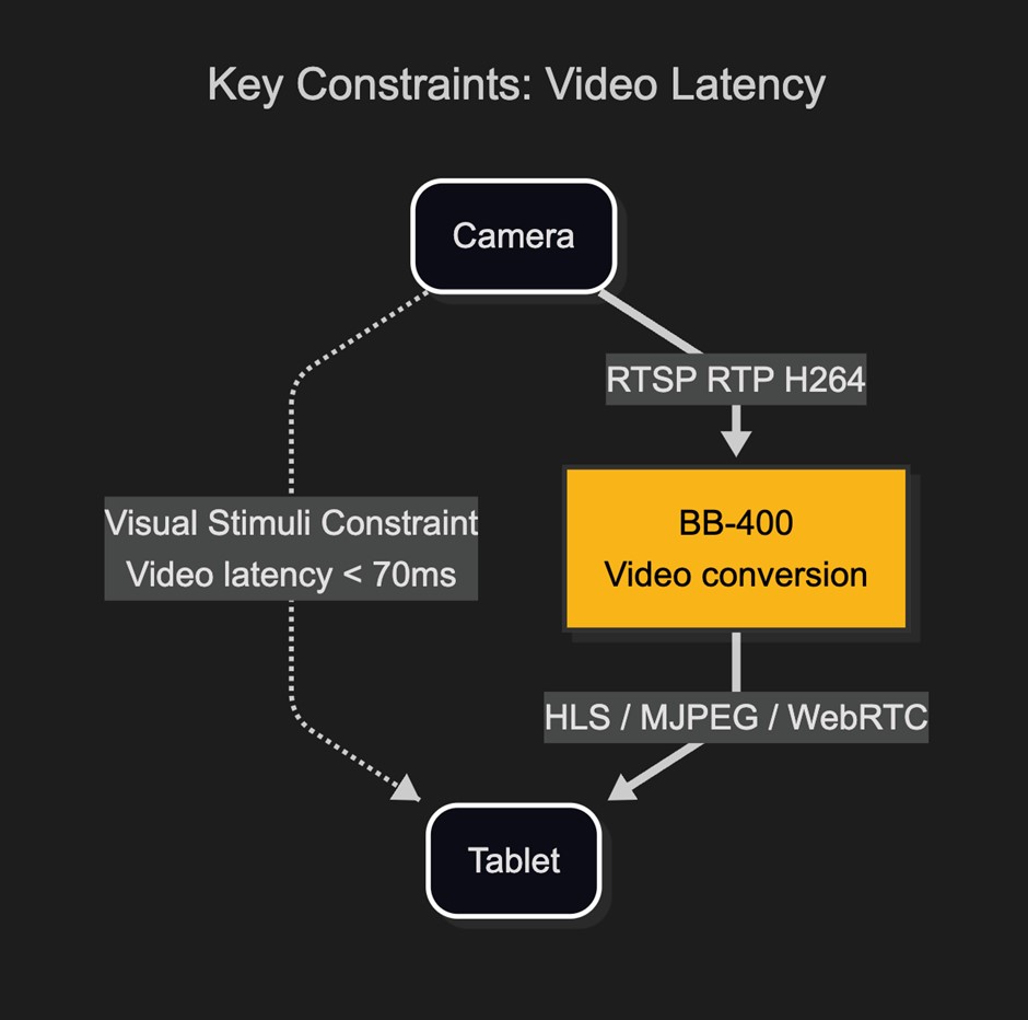
Video latency is the most critical constraint in this real-time system
With the constraint of 70ms latency, several different video streaming options were tested. The video comes from the IP Camera using RTSP protocol and must be converted to a format which can be viewed in a web browser.
The following methods were tested, prioritising simplicity while still meeting the key latency constraint for AI vision systems:
- MJPEG – Motion JPEG: a video compression format where each video frame is a JPEG image and is streamed to the browser in quick succession.
- HLS – HTTP Live Streaming: a video streaming format, where a video stream is broken down into multiple short segments, and sent to a web browser using HTTP.
- WebRTC – Web Real-Time Communication: the most complicated of the options, a public signalling server acts as a gateway to help 2 peers discover the best route over a network to each other. Once the peers have securely verified each other and the best route then an RTP video stream is transmitted.
In all of the examples above, the BB-400 acts as a proxy for the camera stream. Source code for each of the 3 options is available to download and run. The MPJEG and HLS examples use Python, Flask and FFmpeg. For the 3rd option WebRTC (an excellent opensource project), RTSP2WebRTC was used, written in Go, it can be downloaded and complied to target the BB-400.
FFmpeg
FFmpeg (Fast Forward MPEG) is a popular open-source audio visual conversion command line tool available for most platforms. To install on the BB-400 and have the correct hardware acceleration options available do the following on the command line:
sudo apt install ffmpeg
sudo usermod -a -G video bb
Note: The second line is essential to allow FFmpeg access to the hardware decoders.
MJPEG
Taking advantage of the Video 4 Linux hardware decoding support in the BB-400 for H264 video streams, FFmpeg was used to receive the RTSP video stream, decode and then encode as MJPEG.
The FFMPEG command used is:
ffmpeg -c:v h264_v4l2m2m -i RTSP_URL -c:v mjpeg -q:v 10 -f mpjpeg -
The command options can be broken down as follows:
– -c:v h264_v4l2m2m # Use hardware decoding targeting BB-400 CM3+
– -I RTSP_URL # where RTSP_URL is the url of the RTSP camera feed
– -c:v mjpeg # encode output as mjpeg
– -q:v 7 # lower quality to reduce CPU usage but increased data rate
– -f mpjpeg # wrap encoded output in mpjpeg container
– - #output to stdout
Setting the output frame-rate to lower than the input was tested but not found to improve performance. (Using option -frame-rate 10). A gotcha not documented in the FFMPEG docs is that the mpjpeg (Multi-part JPEG) frame boundary used by the encoder uses the label “ffmpeg”.
The output was then streamed using the Flask web-server to the browser. Ultimately the best latency this process allowed for was approx. 1.5 seconds, much too slow to fool human perception that the stream was ‘real-time’.
HLS
HLS, a video protocol introduced by Apple, takes a video stream and slices it into multiple ‘chapters’ (or segments). These chapters are then seamlessly stitched back together at the web-client. One big advantage of HLS over MJPEG is H264 can be used as the video compression format, the same format used by RTSP camera feed, we are simply changing the video container from RTP to HLS. This means very little processing of any kind is required on the BB-400, encoding into H264 is handled by the web camera and decoding to a video happens in the browser. The encoded data is simply copied in and out by the BB-400 over the network.
Again, FFmpeg was used to achieve this, the command used is:
ffmpeg -I RTSP_URL -c:v copy -hls_time 1-hls_list_size 1-tune lowlatency -hls_flags delete_segments+append_list /tmp/stream.m3u8
The command options can be broken down as follows:
– -i RTSP_URL # take the incoming camera feed
– -c:v copy # do not decode, simply copy the data
– -hls_time 1 # set each hls segment length to 1 second
– -hls_list_size 1 # set maximum number of playlist entries to 1
– -tune lowlatency # Tune for low latency
– -hls_flags delete_segments+append_list # delete old and append new segments
– '/tmp/stream.m3u8' # temp location to save the playlist file
The benefit of this approach over MJPEG is that the stream resolution could be higher, as no encoding or decoding was required on the edge device. However, the latency was between 3–5 seconds due to buffering in the web client and the playlist.
WebRTC
WebRTC is a standard for streaming between peers to a web browser. It’s used by many modern conferencing tools like Zoom, Teams and WhatsApp. It was developed and originally released by Google in 2011 and since been adopted as an official standard.
WebRTC was the final option considered due to its complexity. After HLS and MJPEG were shown to have much too high latency, this was the only viable option.
WebRTC uses a signalling server, this is a server at an IP address which can be reached by all peers. The signalling server allows each peer to discover the other and to securely negotiate what media can be sent or received (using SDP – Session Description Protocol). Optionally using STUN (Session Traversal Utilities for NAT) servers, the best route through the network can be discovered to stream data from one peer to the other. Once a route has been found one peer can broadcast an RTP video stream to the other.
A great overview of the implementation details of the standard can be found here.
WebRTC is currently not supported by FFmpeg (although there is an outstanding Pull Request from 2023). After numerous failed attempts to write our own WebRTC implementation an opensource project ‘RTSPtoWebRTC’ by Argentine developer Andrey Semochkin, was used to accomplish the WebRTC server.
Written in programming language Go, the latency of the implementation is under 100ms and uses very low CPU, as again the H264 encoded RTP stream from the camera is simply copied and rebroadcast. At the client side a familiarity with JavaScript is helpful to adapt the code to our demo use case. More info here.
Video Pipeline: Conclusion
WebRTC had by far the lowest latency and allowed for 4k streaming. The main drawback is the complexity of configuration, however using ‘RTSPtoWebRTC’ project handled much of the complexity, acting as both the signalling server and the camera peer, leaving just the front-end integration.
| Protocol | Encoding | Container | CPU/GPU usage | Max resolution | Latency |
| MJPEG | JPEG | MPJPEG | Medium | 640×480 | 1-2 s |
| HLS | H264 | MPEG-2 Transport Stream (TS) | Low | 1920×1080 | 3-5 s |
| WebRTC | H264 | RTP | Low | 3840×2160 | <100ms |
Part 3: AI Vision Systems – Real-World Industrial Applications
Traditionally, vision systems in manufacturing have been used for basic inspection tasks. Relying on pre-programmed rules and fixed algorithms, they can be highly effective in controlled environments where lighting, materials, and part shapes remain consistent, but are far less suited to complex or changing conditions.

This AI vision system game demo highlights how systems that combine affordable edge computing hardware, robust open-source AI tools like LiteRT, and efficient video processing techniques like WebRTC can be scaled and adapted to solve complex engineering challenges across industry.
The technology also enables highly detailed inspections, detecting subtle defects like hairline cracks in metal components, flaws that would typically go unnoticed by traditional inspection methods.
- Defect detection: Imagine an assembly line where every product passing by is instantly analysed for defects. An AI system trained to identify anomalies can trigger alerts, halt production, or even automatically remove flawed items, significantly reducing waste and improving quality control.
- Occupancy and flow monitoring: In a busy warehouse, AI vision can track the movement of goods, monitor worker activity, and optimise traffic flow, increasing efficiency, and improving safety and resource allocation.
- Robotic feedback and guidance: For robotic tasks requiring precision, AI vision can provide real-time feedback. A robot arm can adjust its movements based on visual input, making it more adaptable and efficient.
- Overall Equipment Effectiveness (OEE) measurement: By analysing video streams of machinery and production lines, AI can automatically count parts, detect downtime events, and measure cycle times. This non-intrusive data collection provides valuable insights into OEE without the need for manual data entry or specialist sensors.
Get the code here: https://github.com/brainboxes/brainboxes-edge-ai-vision-demo
-
BB-400
£438.90 Add to cart -
SW-584
£89.00 Add to cart -
SW-595
£179.00 Add to cart